Other signals used for illustration in the article:
Noise,
SinDir;
speech.
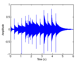
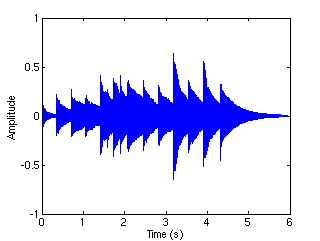
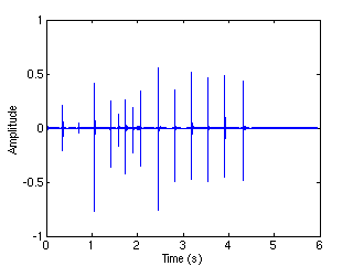
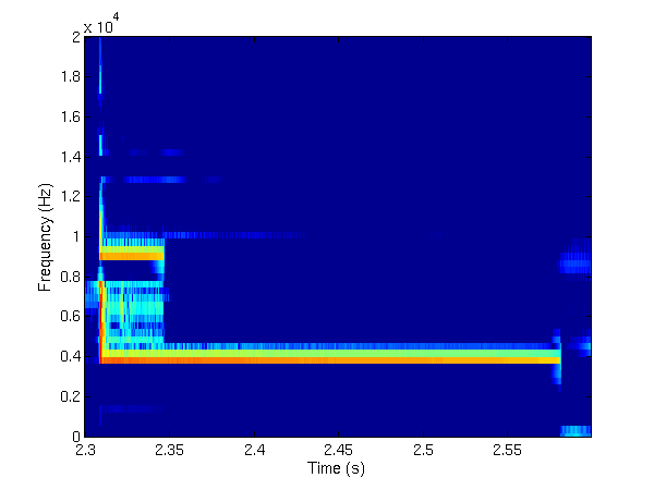
Example of the short
piece of speech signal:
This example was generated using the variant
TFJP1b of the algorithm, which
decomposes the signal into three layers: the tonal layer, i.e.
the component of the signal that is sparsely represented by a Gabor
system with wide windows, the transient layer, i.e. the component that
is sparsely represented by a Gabor system with narrow windows, and the
residual layer, i.e. the component that is not significantly sparsely
represented by either the two systems.
Speech 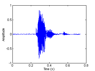 Tonal
Tonal 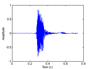 Transient
 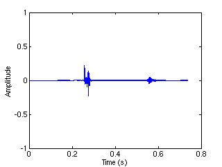 Residual
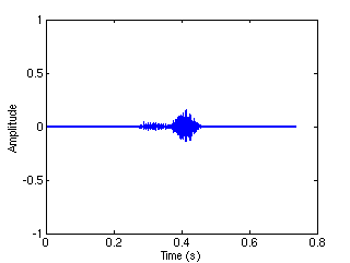
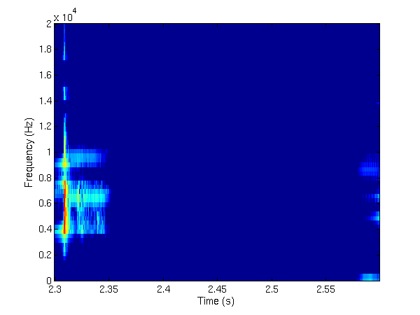
Comparison of the
time-frequency representations obtained with TFJP1 and TFJP2:
In
TFJP1, the super-tiles
corresponding to the two windows are selected at the same time, and the
corresponding signal components are also reconstructed simultaneously.
In
TFJP2, a first set of
super-tiles (corresponding to the first Gabor system) is estimated and
the corresponding component of the signal is reconstructed; then the
second set of super-tiles (corresponding to the second Gabor system) is
selected from the residual, and the corresponding component of the
signal is reconstructed. The procedure is then iterated until the
precision is satisfactory. TFJP2 suffers from smaller "interferences"
between the two components.
TFJP1 and
TFJP2 were run on the same signal,
namely the Glockenspiel signal (Glock, see the examples above). Below
are displayed the time-frequency representations of the "transient
layer" obtained using
TFJP1
and
TFJP2 respectively. As
may be seen from the two time-frequency images, TFJP1 couldn't avoid
selecting one of the harmonic components of the signal, while TFJP2 was
more precise from this point of view.
TFJP1
TFJP2